Real Estate Prediction Using Boosting Tree (XGBoost)

Introduction

The market historical data set of real estate valuation are collected from Xindian Dist., New Taipei City, Taiwan. This project aims to predict price of houses in Xindian, New Taipei given some characteristics of buildings.

Xindian, New Taipei City,Taiwan

The Data

This data is available in the public and is collected from UC Irvine Machine Learning Repository, for more data to practice machine learning visit UCirvine.

real_estate <- read_excel("Real estate valuation data set.xlsx") |> 
  clean_names()

head(real_estate)

# A tibble: 6 × 8
     no x1_transaction_date x2_house_age x3_distance_to_the_nearest_mrt_station
  <dbl>               <dbl>        <dbl>                                  <dbl>
1     1               2013.         32                                     84.9
2     2               2013.         19.5                                  307. 
3     3               2014.         13.3                                  562. 
4     4               2014.         13.3                                  562. 
5     5               2013.          5                                    391. 
6     6               2013.          7.1                                 2175. 
# ℹ 4 more variables: x4_number_of_convenience_stores <dbl>, x5_latitude <dbl>,
#   x6_longitude <dbl>, y_house_price_of_unit_area <dbl>

Data Definition

Variable Name	Role	Type	Description	Units	Missing Values
No	ID	Integer			no
X1	transaction date	Feature	Continuous	for example, 2013.250=2013 March, 2013.500=2013 June, etc.	no
X2	house age	Feature	Continuous		year
X3	distance to the nearest MRT station	Feature	Continuous		meter
X4	number of convenience stores	Feature	Integer	number of convenience stores in the living circle on foot	integer
X5	latitude	Feature	Continuous	geographic coordinate, latitude	degree
X6	longitude	Feature	Continuous	geographic coordinate, longitude	degree
Y house price of unit area	Target	Continuous	10000 New Taiwan Dollar/Ping, where Ping is a local unit, 1 Ping = 3.3 meter squared	10000 New Taiwan Dollar/Ping	no

Data Preparation

First, we will split the date from the Taiwan system to year and month.

real_estate <- real_estate |> 
  mutate(
    year = x1_transaction_date %/% 1,
    month = round((x1_transaction_date %% 1) * 12), # to get month from taiwanese date
    .before = x2_house_age
  )


real_estate <- real_estate |> 
  mutate(month = case_when(month == 0 ~ 1, TRUE ~ month)) |> 
  select(!c(1, 2))

The names of the variables are a bit long and unclear so we will rename them to make coding easy

real_estate <- real_estate |> 
  rename(
    age = x2_house_age,
    distance_to_station = x3_distance_to_the_nearest_mrt_station,
    number_convenience_stores = x4_number_of_convenience_stores,
    latitude = x5_latitude,
    longitude = x6_longitude,
    price = y_house_price_of_unit_area
  )

real_estate <- real_estate |> 
  mutate(
    age = ceiling(age),
    sale_date = make_date(year = as.integer(year), month = month),
    .before = age
  ) |> 
  select(-c(year, month))

names(real_estate)

[1] "sale_date"                 "age"                      
[3] "distance_to_station"       "number_convenience_stores"
[5] "latitude"                  "longitude"                
[7] "price"                    

To get a better grasp of the pricing, the US Dollar will be used, and the size of the houses in square meter will be calculated to give an idea of how big the properties are

real_estate <- real_estate |> 
  mutate(
    size_m2 = (price * 10000) / 3.9,
    price_usd = (price * 10000) * 0.032,
    .before = price
  )

Missing values??

Even if the data is having no missing value when imported, it’s not a bad idea to look for missing data after the preparation which we have made.

sum(is.na(real_estate))

[1] 0

We can also check for duplicate data point

sum(duplicated(real_estate))

[1] 0

There are no duplicate data point. We can proceed with our analysis after this.

Exploratory Data Analysis

Target Variable

Univariate

price_median <- 
  tibble(
    med = median(real_estate$price_usd),
    label = paste0("$", med)
  )

ggplot(real_estate, aes(price_usd)) +
  geom_histogram(binwidth = 500, alpha =0.7, fill = "wheat3") +
  geom_density(stat = "bin", binwidth = 500, col = "brown") +
  geom_vline(aes(xintercept = median(price_usd)), col = "violetred3") +
  geom_text(
    data = price_median,
    aes(x = med, y = 30, label = label),
    hjust = -0.3,
    col = "red"
  ) +
  labs(
    x = "Price",
    y = "count",
    title = "Long-tailed Price distribution"
  ) +
  theme_igray() +
  scale_x_continuous(label = label_dollar())

Figure 1: House price distribution

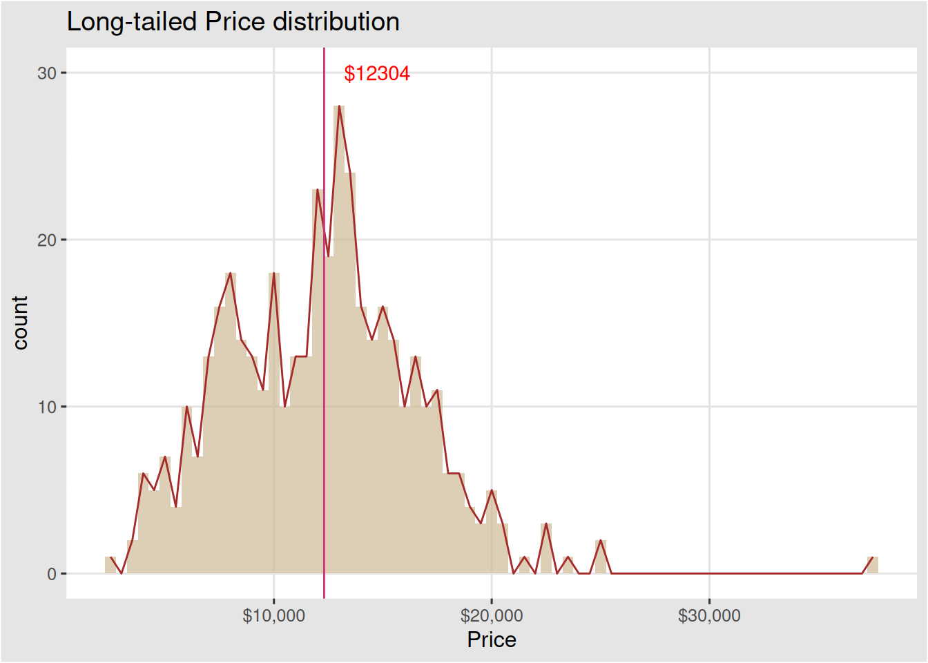
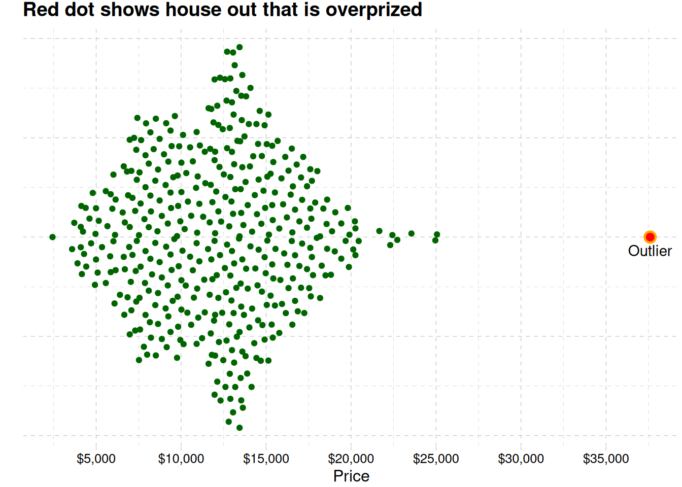
The most house price ranges between 11000 to 14000 dollars Figure 1. The distribution shows there seems to be an outlier in our data. fig-outlier shows the outlier

outlier <- 
  tibble(
    x = 1,
    max_price = max(real_estate$price_usd),
  )

    
ggplot(real_estate, aes(price_usd, x = 1)) +
  ggbeeswarm::geom_quasirandom(
    col = "darkgreen",
    shape = "circle"
  ) + 
  geom_point(
    data = outlier, 
    aes(x, max_price),
    shape = "circle filled", stroke = 1.2, size = 3,
    fill = "red",  col = "orange",
  ) +
  geom_text(
    data = outlier,
    aes(y = max_price, label = "Outlier"),
    vjust = 1.7
  ) +
  scale_y_continuous(
    label = label_dollar(),
    breaks = seq(0, 40000, 5000)
  ) +
  labs(
    x = "",
    y = "Price",
    title = "Red dot shows house out that is overprized"
  ) +
  coord_flip() +
  theme(
    axis.text.y = element_blank(),
    axis.ticks.y = element_blank(),
    axis.title.y = element_blank()
  ) +
  theme_pander()

Figure 2: Outlier point significantly overprized above 30000 usd

We need to remove the overprized house

real_estate <- real_estate |> filter(!price_usd > 30000)

range(real_estate$price_usd)

[1]  2432 25056

We will continue our EDA now that the outlier has been removed

Multivariate

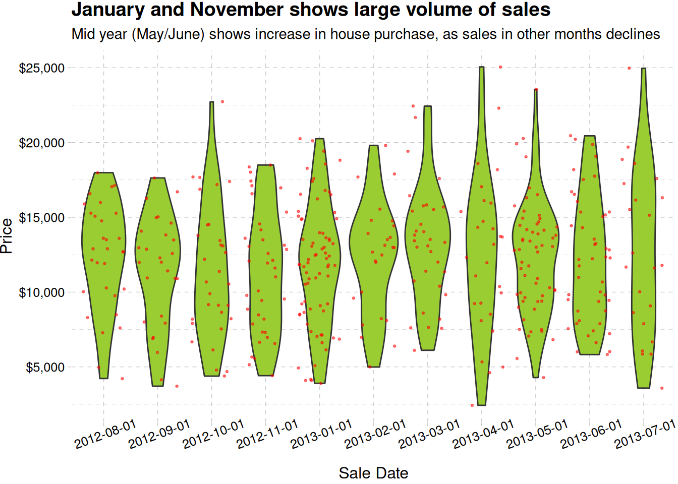
ggplot(real_estate, aes(factor(sale_date), price_usd)) +
  geom_violin(fill = "olivedrab3") +
  geom_jitter(aes(y = price_usd), size = 0.5, alpha = 0.5, col = "red") +
  theme(axis.text.x = element_text(angle = 20)) +
  labs(x = "Sale Date", y = "Price", 
       title = "January and November shows large volume of sales",
       subtitle = "Mid year (May/June) shows increase in house purchase, as sales in other months declines"
  ) +
  scale_y_continuous(label = label_dollar()) +
  theme_pander()

Monthly price distribution of houses, there are some traces of seasonality

m

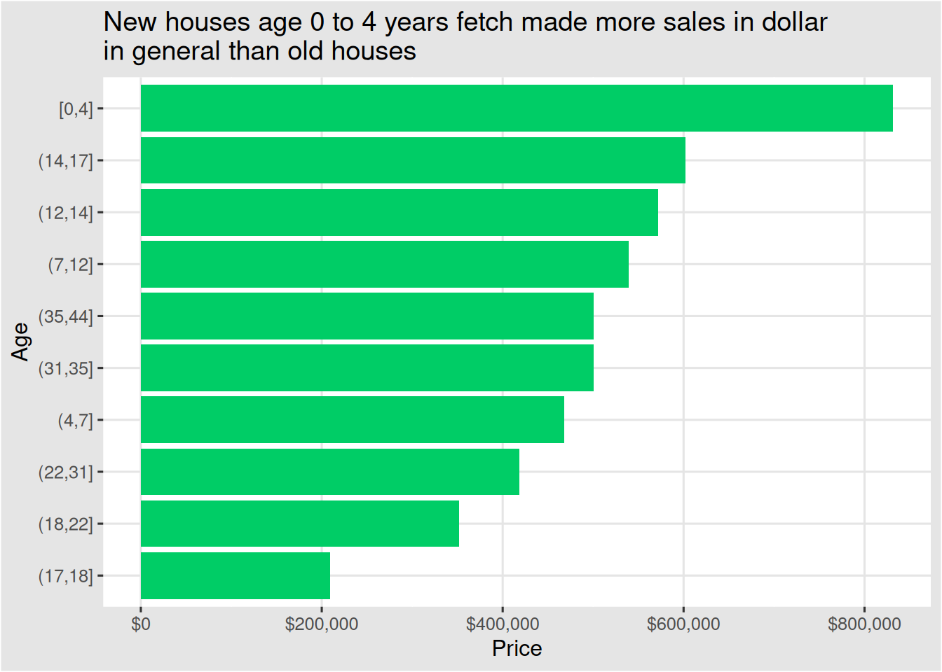
ggplot(real_estate, aes(fct_reorder(cut_number(age, 10), price_usd, .fun = sum), price_usd)) +
  geom_col(fill = "springgreen3") +
  labs(
    x = "Age",
    y = "Price",
    title = str_wrap("New houses age 0 to 4 years fetch made more sales in dollar
                     in general than old houses", width = 60)
  ) +
  scale_y_continuous(label = label_dollar()) +
  coord_flip() +
  theme_igray()

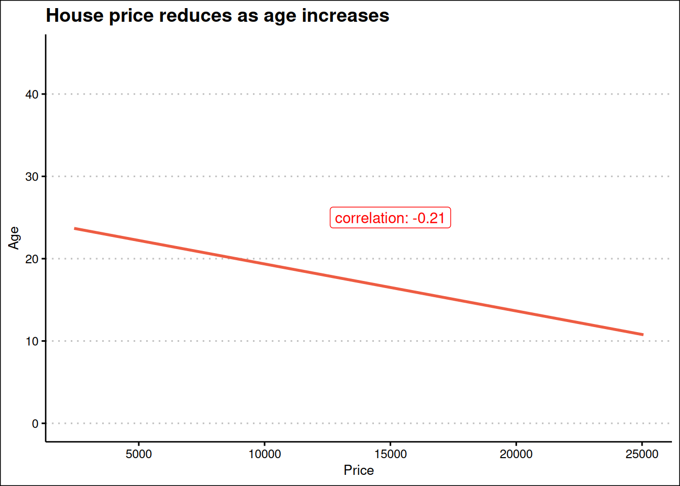
correlation <- cor(real_estate$price_usd, real_estate$age)

ggplot(real_estate, aes(price_usd, age)) +
  geom_smooth(method = "lm", se = F, col = "tomato2") +
  expand_limits(y = c(0, 45)) +
  labs(
    x = "Price",
    y = "Age",
    title = "House price reduces as age increases"
  )+
  annotate(
    geom = "label",
    label = paste("correlation:", round(correlation, 2), sep = " "),
    x = 15000, y = 25, col = "red"
  ) +
  theme_clean()

`geom_smooth()` using formula = 'y ~ x'

Figure 3: Correlation between age and price

Figure 3 shows the relationship between house price and the age of houses

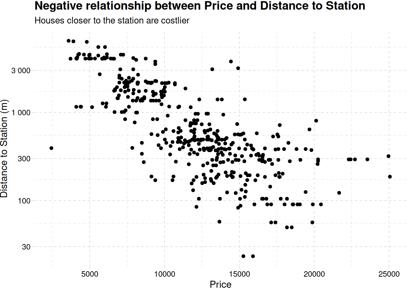
ggplot(real_estate, aes(price_usd, distance_to_station)) +
  geom_point() +
  scale_y_log10(label = label_number()) +
  labs(
    x = "Price",
    y = "Distance to Station (m)",
    title = "Negative relationship between Price and Distance to Station",
    subtitle = "Houses closer to the station are costlier"
  ) +
  theme_pander()

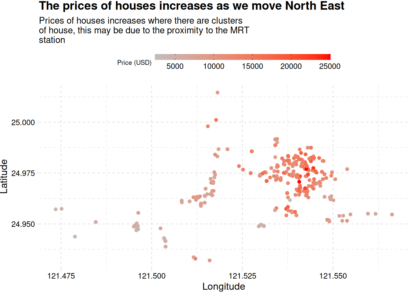
ggplot(real_estate, aes(longitude, latitude, col = price_usd)) +
  geom_jitter() +
  labs(
    col = "Price (USD)",
    x = "Longitude",
    y = "Latitude",
    title = "The prices of houses increases as we move North East",
    subtitle = str_wrap("Prices of houses increases where there are clusters\ of house, this
                        may be due to the proximity to the MRT station", width = 55)
  ) +
  scale_colour_gradient(low = "gray", high = "red") +
  theme_pander() +
  theme(legend.position = "top") +
  guides(
    color = guide_colorbar(barwidth = 15, barheight = 1/2, ticks.colour = "black", title.position = "left", title.theme = element_text(size = 8)))

Houses get expensive as we move in a northeast direction,

Correlation with other variables

ggcorr(real_estate |> select(!c(sale_date, price)))

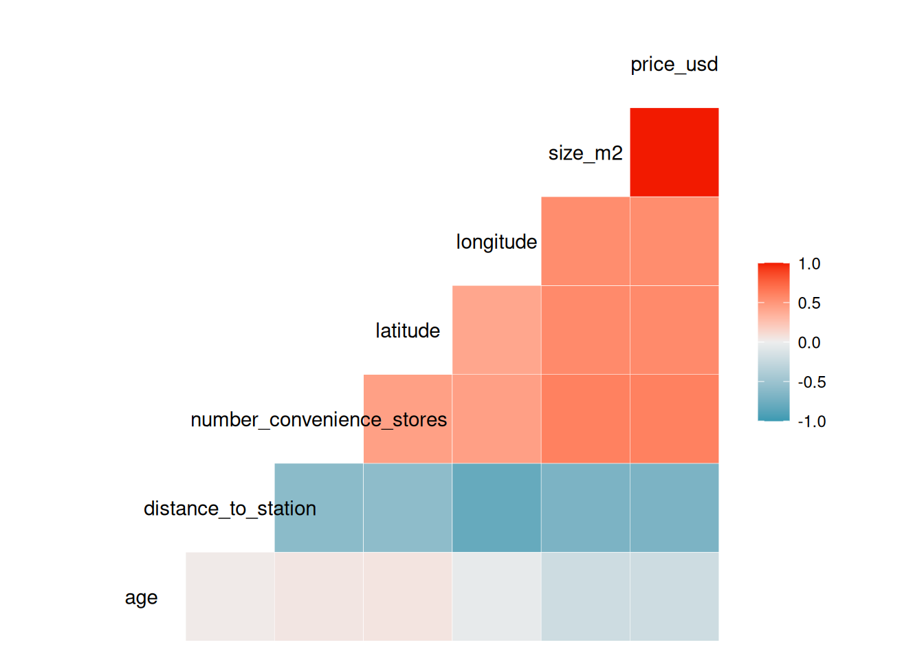
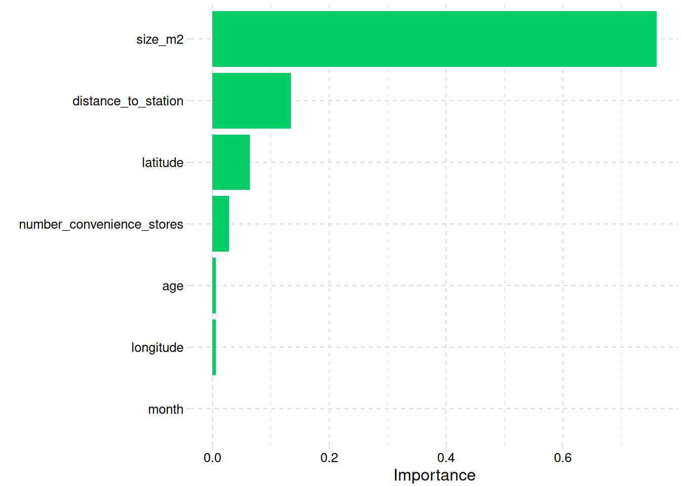
All the factors shows strong relationship with the price of the building

While size, number of convenience store close to the building and the position of the building, i.e., longitude and latitude are positively correlated to the price of a building, the older a building, and the farther it is from the MRT station the more likely it reduces in price.

Model Building

Before we begin modeling, we need to remove some variables that might not be a big influence, this include:

• sales_date, as there is just a year span of data, it is better we extract just the month use that

• price, we have price in US Dollar, already, we do not need the price in Taiwanese dollars.

real_estate <- real_estate |> 
  mutate(
    month = month(sale_date),
    .before = age
  ) |> 
  select(-c(sale_date, price))

head(real_estate)

# A tibble: 6 × 8
  month   age distance_to_station number_convenience_stores latitude longitude
  <dbl> <dbl>               <dbl>                     <dbl>    <dbl>     <dbl>
1    11    32                84.9                        10     25.0      122.
2    11    20               307.                          9     25.0      122.
3     7    14               562.                          5     25.0      122.
4     6    14               562.                          5     25.0      122.
5    10     5               391.                          5     25.0      122.
6     8     8              2175.                          3     25.0      122.
# ℹ 2 more variables: size_m2 <dbl>, price_usd <dbl>

For this analysis, we will use:

• XGboost

Data Sharing

set.seed(333)


real_estate_split <- initial_split(real_estate, prop = .8, strata = price_usd)

real_estate_train <- training(real_estate_split)
real_estate_test <- testing(real_estate_split)

real_estate_split

<Training/Testing/Total>
<328/85/413>

Model Specification

Given our choice of model, XGBoost, a tree-based model, a lot of preprocessing is not required, we can going to dive right into our model specification, and tune a lot of the model hyperparameter to reduce the chances of over-fitting and under-fitting.

xg_model <- 
  boost_tree(
    mtry = tune(), min_n = tune(),
    tree_depth = tune(), trees = 1000,
    loss_reduction = tune(),
    sample_size = tune(),
    learn_rate = tune(),
  ) |> 
  set_engine("xgboost") |> 
  set_mode("regression")

xg_model |>  translate()

Boosted Tree Model Specification (regression)

Main Arguments:
  mtry = tune()
  trees = 1000
  min_n = tune()
  tree_depth = tune()
  learn_rate = tune()
  loss_reduction = tune()
  sample_size = tune()

Computational engine: xgboost 

Model fit template:
parsnip::xgb_train(x = missing_arg(), y = missing_arg(), weights = missing_arg(), 
    colsample_bynode = tune(), nrounds = 1000, min_child_weight = tune(), 
    max_depth = tune(), eta = tune(), gamma = tune(), subsample = tune(), 
    nthread = 1, verbose = 0)

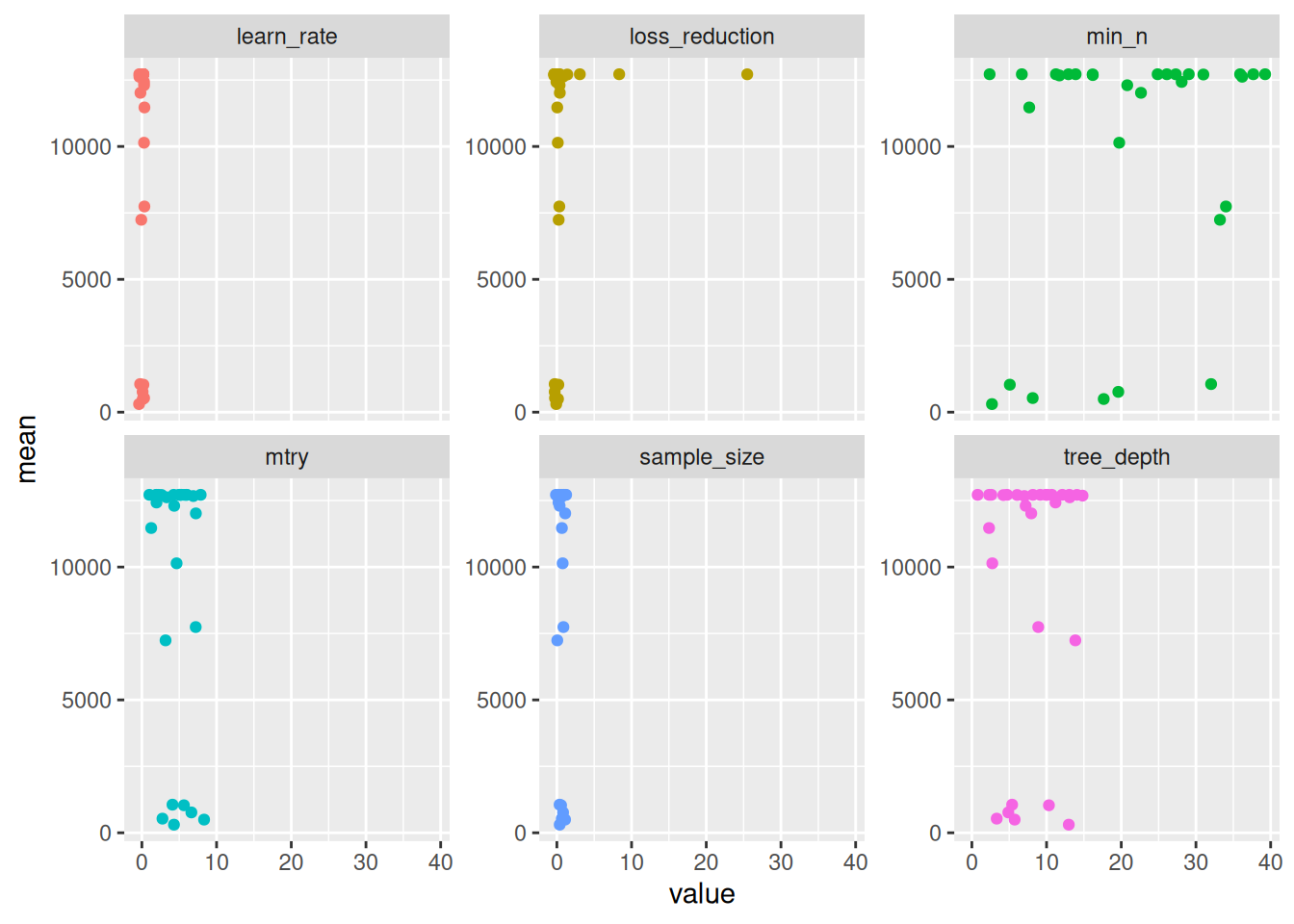
Tune Grid

Next, we have to set up some values for our hyperparameter, we don’t want to exhaust our computing resource, and face the risk of overfitting. We will use the Latin Hypercube grid as this approach can be more computationally efficient than a regular grid, especially when there are many hyperparameters to tune. Random selection can also introduce diversity into the search process.

set.seed(3434)


xgb_grid <- grid_latin_hypercube(
  tree_depth(),
  min_n(),
  loss_reduction(),
  sample_size = sample_prop(),
  finalize(mtry(), real_estate_train),
  learn_rate(),
  size = 30
)

xgb_grid

?(caption)

# A tibble: 30 × 6
   tree_depth min_n loss_reduction sample_size  mtry learn_rate
        <int> <int>          <dbl>       <dbl> <int>      <dbl>
 1          5    32       1.17e- 6       0.529     4   8.06e- 3
 2          6    16       3.05e- 1       0.446     3   5.03e- 7
 3         15    16       3.58e- 9       0.566     2   2.56e- 6
 4         13    36       5.57e- 1       0.637     3   7.82e- 6
 5         10     7       2.58e- 4       0.668     5   7.03e-10
 6          5    20       1.11e- 2       0.491     7   5.75e- 3
 7          8    13       3.64e-10       0.339     6   1.05e- 7
 8         13    25       2.87e+ 0       0.937     1   2.94e-10
 9          4    31       1.55e+ 0       0.827     2   8.75e- 7
10          5    14       7.17e- 4       0.771     5   1.64e-10
# ℹ 20 more rows

Since mtry depends on the number of predictors, it had to be tuned differently ?@tbl-boost-tree-grid.

Workflow Process

To improve efficiency and streamline processes, we start a modelling workflow.

xg_wf <- workflow() |> 
  add_formula(price_usd ~ .) |> 
  add_model(xg_model)

xg_wf

══ Workflow ════════════════════════════════════════════════════════════════════
Preprocessor: Formula
Model: boost_tree()

── Preprocessor ────────────────────────────────────────────────────────────────
price_usd ~ .

── Model ───────────────────────────────────────────────────────────────────────
Boosted Tree Model Specification (regression)

Main Arguments:
  mtry = tune()
  trees = 1000
  min_n = tune()
  tree_depth = tune()
  learn_rate = tune()
  loss_reduction = tune()
  sample_size = tune()

Computational engine: xgboost 

Cross Validation

Next, we create resamples for tuning the model, ?@tbl-cross-validation-resamples.

set.seed(222)

real_estate_folds <- vfold_cv(real_estate_train, strata = price_usd)

?(caption)

NOW WE TUNE. We will use our resamples, the tuneable workflow, and the Latin grid of parameters which we have to try get the best value. To also speed up the process, we will enable parallel computing

doParallel::registerDoParallel()

set.seed(222)

xg_tune_res <- tune_grid(
  xg_wf,
  resamples = real_estate_folds,
  grid = xgb_grid,
  control = control_grid(save_pred = T)
)

Exploring Tune Results

xg_tune_res |> 
  collect_metrics() |> 
  filter(.metric == "rmse") |> 
  select(mean, mtry:sample_size) |> 
  pivot_longer(
    mtry:sample_size,
    values_to = "value",
    names_to = "parameter"
  ) |> 
  ggplot(aes(value, mean, color = parameter)) +
  geom_jitter(show.legend = F, width = .4) +
  facet_wrap(~parameter, scales = "free_y")

The lower the rmse, the better the model, a simplification, but this is not always the case. We will stick to that for now.

Let’s show the best performing set of parameter ## Best Tune

show_best(xg_tune_res, metric = "rmse")

# A tibble: 5 × 12
   mtry min_n tree_depth learn_rate loss_reduction sample_size .metric
  <int> <int>      <int>      <dbl>          <dbl>       <dbl> <chr>  
1     4     3         13    0.0145     0.0000176         0.704 rmse   
2     8    18          6    0.0578     0.0000239         0.966 rmse   
3     3     8          3    0.0422     0.00411           0.688 rmse   
4     7    20          5    0.00575    0.0111            0.491 rmse   
5     6     5         10    0.00269    0.000000326       0.893 rmse   
# ℹ 5 more variables: .estimator <chr>, mean <dbl>, n <int>, std_err <dbl>,
#   .config <chr>

Finalize Model Workflow

Let’s select the best and use it to finalize our model.

Select Best Parameter

best_rmse <- select_best(xg_tune_res, "rmse")
best_rmse

# A tibble: 1 × 7
   mtry min_n tree_depth learn_rate loss_reduction sample_size .config          
  <int> <int>      <int>      <dbl>          <dbl>       <dbl> <chr>            
1     4     3         13     0.0145      0.0000176       0.704 Preprocessor1_Mo…

Now we can finalize the model

final_boost_tree <- finalize_workflow(
  xg_wf,
  best_rmse
)

final_boost_tree

══ Workflow ════════════════════════════════════════════════════════════════════
Preprocessor: Formula
Model: boost_tree()

── Preprocessor ────────────────────────────────────────────────────────────────
price_usd ~ .

── Model ───────────────────────────────────────────────────────────────────────
Boosted Tree Model Specification (regression)

Main Arguments:
  mtry = 4
  trees = 1000
  min_n = 3
  tree_depth = 13
  learn_rate = 0.0145039211746767
  loss_reduction = 1.76136801549921e-05
  sample_size = 0.70429474228993

Computational engine: xgboost 

Variable Importance

Let’s see the most important variables in the model.

library(vip)

Attaching package: 'vip'

The following object is masked from 'package:utils':

    vi

final_boost_tree |> 
  fit(data = real_estate_train) |> 
  pull_workflow_fit() |> 
  vip(
    geom = "col",
    aesthetics = list(fill = "springgreen3")
  ) +
  theme_pander()

Warning: `pull_workflow_fit()` was deprecated in workflows 0.2.3.
ℹ Please use `extract_fit_parsnip()` instead.

The most important predictor of the price of a house are the:

• Size
• Distance to the station,
• The latitude of the buildings, and
• The number of convenience stores.

Model Test

Let’s test how good the model is with the test data.

final_result <- last_fit(final_boost_tree, real_estate_split)

collect_metrics(final_result)

# A tibble: 2 × 4
  .metric .estimator .estimate .config             
  <chr>   <chr>          <dbl> <chr>               
1 rmse    standard     177.    Preprocessor1_Model1
2 rsq     standard       0.998 Preprocessor1_Model1

That’s a high Rsquared, close to 1, and the RMSE have a very low error of ± 225.4 dollars. Let’s plot prediction vs actual values

final_result |> 
  collect_predictions() |> 
  select("actual" = price_usd, "prediction" = .pred) |> 
  ggplot(aes(actual, prediction)) +
  geom_point(col = "orange2") +
  geom_label(
    aes(x = 10500, y = 15000, label = "R-square: 0.9974"),
    col = "blue"
  ) +
  geom_abline(col = "red") +
  theme_few()

The plot shows a good performance of the model. For future prediction on a similar data in the region we extract the model and save it for later use.

real_estate_boost_tree_model <- final_result |> 
  extract_fit_parsnip()

# Conclusion

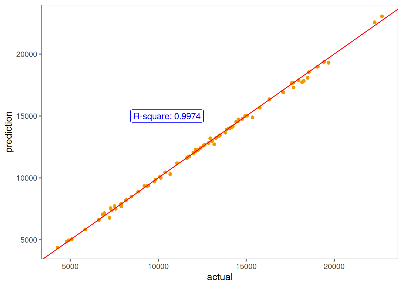
This project shows the capabilities of R, and the XGBoost algorithm in real estate use. While the model was built to predict price, it could be made better if a time component is give. Given the data used for this project, a time component is ill-advised as seasonality, and other time related components will not be properly studied by the algorithm.

Back to homepage